
V 1.0 The Covid-19 Pandemic: Basic Insights from Basic Mathematical Models
Abstract
Mathematical models for the spread of infectious diseases have a long history. From the start of the Covid-19 pandemic, there was a huge public interest in applying such models, since they help to understand general features of epidemic spread and support the assessment of possible mitigation measures – and their later relaxation. We describe and discuss some well-established mathematical models for epidemic spread, starting from the susceptible-infected-recovered (SIR) model and branching processes and discussing insights from network-based models. During the Covid-19 pandemic, such classical models have also been extended to include many additional aspects that affect epidemic spread, such as mobility patterns or testing possibilities. However, such complex models are increasingly difficult to assess from the outside. In a situation where their predictions can directly affect the lives of millions of people, this can become a severe problem. We argue that simple mathematical models have huge merits and can explain many of the key features of more complex models, such as the importance of heterogeneity in disease transmission. For example, basic models allow inferring whether super-spreading, where very few infected individuals cause the vast majority of secondary cases, should be the rule or the exception – with wide-ranging consequences for the possible success of mitigation measures. In addition, these basic models are simple enough to be understood and implemented without expert knowledge in theoretical epidemiology or computer science. Thus, they offer a level of transparency that can be important for a society to accept mitigation measures.
General Lay Summary
During the Covid-19 pandemic, scientists have been describing the spread of the virus with different kinds of theoretical models. While some of these models are challenging to understand in detail, they typically are based on a core of a few classical epidemiological models that are also accessible to non-experts. In this article, we discuss several of these classical models and highlight important conclusions that can be drawn from them. We are convinced that an understanding of these models can crucially contribute to the public acceptance of governmental interventions and to more informed discussions about upcoming decisions. The media often depicts mathematical models as complicated black boxes that only a few experts can master. While the development and analysis of mathematical models indeed requires the expertise of specialists, we believe that our society can understand many aspects of these models and of the theoretical basics of infectious disease dynamics.
Generelle Zusammenfassung
Während der Covid-19-Pandemie haben Wissenschaftler die Ausbreitung des Virus mit unterschiedlichen theoretischen Modellen beschrieben. Auch wenn einige dieser Modelle im Detail nur schwer zu verstehen sind, basieren sie typischerweise auf wenigen klassischen epidemiologischen Modellen, die auch für Nicht-Experten verständlich sind. In diesem Artikel diskutieren wir einige dieser klassischen Modelle und heben wichtige Schlussfolgerungen hervor, die aus ihnen gezogen werden können. Wir sind davon überzeugt, dass das Verstehen dieser Modelle entscheidend zur öffentlichen Akzeptanz staatlicher Interventionen und zu konstruktiven Diskussionen über anstehende Ent¬scheidungen beitragen kann. Die Medien stellen mathematische Modelle oft als komplizierte Black Boxes dar, die nur wenige Experten ver¬stehen können. Auch wenn die Entwicklung und Analyse mathematischer Modelle in der Tat das Fachwissen von Spezialisten erfordert, glauben wir, dass unsere Gesellschaft viele Aspekte dieser Modelle und der theoretischen Grundlagen der Dynamik von Infektionskrankheiten verstehen kann.
Keywords
1. Introduction
These are the days of mathematical biology. A discipline that was sometimes viewed as supporting experimental sciences only, suddenly becomes central and immediately relevant for societies worldwide to plan and assess mitigation measures during the Covid-19 pandemic. Theoretical research about disease spread, contact networks, and models of virus evolution suddenly became part of the general public discussion, the daily media, and the concern of politicians. Many scientists have switched their working and communication style to address important problems arising during the pandemic in a timely manner. What does the public expect from such theoretical models? Some would like to have a precise prediction of the future – and as long as the predictions are sufficiently accurate, they tend to care less about the underlying model. Others would like to understand the underlying mechanisms, allowing them to think carefully about possible interventions and work with different future scenarios. The purpose of the model has to be taken into account already when the model is developed, as different purposes can call for different kinds of models (Holmdahl and Buckee 2020).
The subject of mathematical modeling of epidemic spread has a very long history (Bernoulli 1766, Ross 1908, Kermack and McKendrick 1927). Infectious disease dynamics has been the focus of a major part of this field, and many mathematical biologists have worked towards understanding and predicting the possible courses of diseases such as influenza or HIV for decades. In a time when every national (and often also regional) government is forced to take wide-ranging decisions that temporarily affect their citizens’ daily lives, there was a high demand for the expertise of theoretical epidemiologists (Gog 2020) – and in several countries, not enough epidemiologists were available to meet this demand. During this time, applying well-established models to Covid-19 data was an important contribution to assessing the situation. Thus, many scientists who worked on other subjects before but were well familiar with the underlying theoretical methods have quickly entered the field. While some of this work merely rediscovered established insights or may even be questionable (a particular problem when the public picks up pre-prints), a lot of the work of newcomers proved to be important and meaningful.
Here, we discuss a number of basic mathematical models. These models had been developed much earlier – either to describe other infectious diseases or in terms of the basic understanding of infectious disease dynamics – and have now been used to understand the course of the pandemic. We focus, in particular, on basic models that abstract from many known biological issues but that are ideal for highlighting important points about the dynamics of infectious diseases. Such models are particularly helpful for the general public and decision-makers, as they are transparent and allow us to better understand the typical dynamics of an epidemic. Concepts such as reproductive numbers, herd immunity, or overdispersion that are discussed in the public typically go back to these basic models. A good understanding of such concepts seems to be of immediate value in assessing the situation and discussing the implementation of different mitigation measures – or their relaxation.
2. Classes of Epidemiological Models
In the following, we present four different classes of epidemiological models, starting with the most basic models that describe the dynamics of the number of infected individuals either by deterministic or stochastic processes. Subsequently, we move to models with an explicit contact structure. These first three classes of models build the basis for the subsequent sections. We also briefly discuss complex agent-based models that aim to consider many more factors that could affect the course of an epidemic.
2.1 Deterministic Models: The SIR Model and its Extensions
Mathematical models to describe the spread of infectious diseases have a long history (Bernoulli 1766, Hamer 1906, Ross 1908, 1916, Ross and Hudson 1917a, 1917b, Bernoulli and Blower 2004). The most popular model in this context, the SIR model (“Susceptible-Infected-Recovered”), is usually attributed to Kermack and McKendrick (1927). The model was initially formulated in discrete time and used differential equations as an approximation. Nowadays, the SIR model is usually introduced from the start as a set of differential equations. These describe the change in the number of those who are susceptible, S(t), those who are currently infected, I(t) and those who are recovered, R(t),
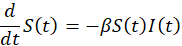 (1a)
(1a)
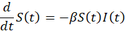 (1b)
(1b)
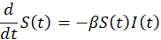 (1c)
(1c)
where the population size N = S(t) + I(t) + R(t) is constant over time. On the left-hand side, we have the temporal change in the number of individuals of a certain type. The first term on the right-hand side of Eqs. (1a) and (1b) describes that susceptible individuals are infected and become infectious themselves, which happens at rate 𝛽S(t)I(t). The second term on the right-hand side of Eq. (1b) describes recovery, which leads to an increase in the number of recovered individuals at rate 𝛾I(t) in Eq. (1c), see Fig. 1A and 1B. As long as the recovery rate is lower than the rate of new infections, 𝛾<𝛽S(t), the number of infected individuals increases. The ratio R0 = S(0)𝛽/𝛾 is often used to characterize the system, where R0 is the so-called basic reproductive number of the epidemic. In an individual-based model, this corresponds to the number of secondary cases caused by one infectious individual in a fully susceptible population: An infected individual on average remains infectious over a time 1/𝛾. During this time, this individual on average infects 𝛽S(0) others, which leads on average to S(0)𝛽/𝛾 secondary cases.
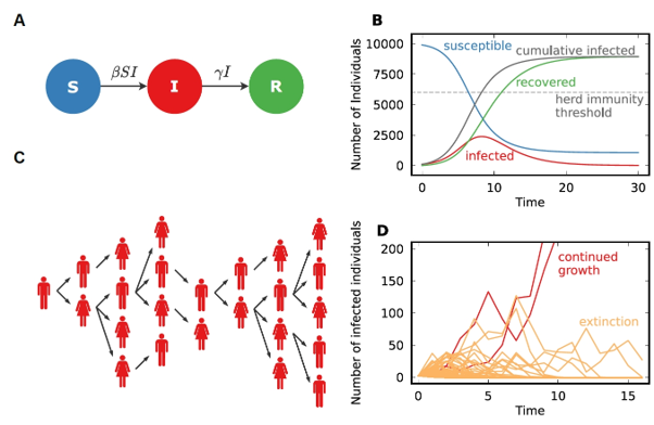
Fig. 1 Illustration of the SIR model and branching processes. (A) shows the basic dynamics turning susceptible individuals (S) at rate 𝛽SI into infected individuals (I). Infected individuals recover at rate 𝛾 I, such that eventually more and more individuals have recovered (R). (B) Temporal dynamics in the SIR model (𝛽 = 1, 𝛾 = 0.4, and N = 10000). The number of infected individuals increases until the condition 𝛽 S(t) = 𝛾 is fulfilled. From then on, the cumulative number of infected individuals has reached the herd immunity threshold. At this point, every infected individual causes on average less than one secondary case, slowing down the epidemic. However, the cumulative number of infected individuals by the end of the pandemic can be much larger than the herd immunity threshold. (C) Illustration of a branching process model, where each infected primary case can cause a variable number of secondary cases. Secondary cases are assumed to be independent for each infected case, which implies that no individual is potentially infected by two primary cases. (D) The branching process ultimately leads either to extinction, where no infected individuals are present anymore, or to a continued increase, which increases on average exponentially. Here we show 50 trajectories, and colors distinguish between those going extinct and those that continue and only go extinct again with a probability < 10−7 (pj given by a negative binomial distribution with basic reproductive number R0 = 2 and dispersion parameter k = 0.2, see main text).
There are numerous extensions of this model, which, e.g., work with additional compartments (e.g., exposed, but not yet infectious, leading to an SEIR model), models with time delays, models with behavioral feedback, or models with more types of infections. In addition, some extensions consider population structure or stochastic effects. In terms of population structure, the SIR model can be viewed as a “mean-field” model, which describes the average dynamics only. Thus, it is based on the underlying assumption that all individuals in the population are identical and, e.g., spread the disease in the same way. While this is, of course, an idealization, it provides a very good approximation of the dynamics for many kinds of population structures.
2.2 Stochastic Models: Branching Processes
The deterministic SIR model introduced in the previous section describes the expected dynamics and does not account for any stochastic effects. Most importantly, it does not account for stochastic variation in the number of secondary cases. This variation can crucially affect the dynamics of the pandemic when case numbers are low and the spread of rare new variants. How much variation there is also influences which control interventions are most effective.
There are many ways to formulate a stochastic version of the SIR model, e.g., by using the rates 𝛽 and 𝛾 to capture the probabilities for individual infection and recovery processes. However, in this section, we will go a different route and instead introduce another class of models – branching process models. Branching processes are stochastic processes making the assumption that individuals cause secondary cases independent from each other (and independent from any past infections in the population). This is a good assumption when case numbers are low. Likewise, it is a good assumption when considering the initial spread of a new virus variant. During the exponential growth phase, a stochastic SIR model can be well described by a branching process, see Fig. 1C and 1D.
We here introduce the classical discrete-time Galton-Watson branching process (Watson and Galton 1875), which allows us to understand some key consequences of stochasticity for disease dynamics. It was originally developed to describe how noble names are passed down to the children. Formulating the definition in terms of disease dynamics, the Galton-Watson branching process is defined by the following assumptions: Each infected individual infects j other individuals according to some probability distribution  with mean R0. This distribution is (i) the same for all infected individuals (ii) independent of the number of infected individuals (iii) independent of the number of secondary cases caused by other individuals (iv) constant over time. Individuals recover after one time unit, and all infections occur right at the end of this time unit.
There are other types of branching processes that better match the dynamics of disease spread, e.g., individuals recover after a variable time period, and infections occur randomly over time. However for many questions, it is irrelevant at which precise time points infections happen, and the relevant behavior is captured well by the Galton-Watson branching process.
In the context of epidemics, a popular choice for the distribution of the number of secondary cases is the negative binomial distribution (Lloyd-Smith et al. 2005). The reasoning behind this choice is that individuals have an “individual basic reproductive number”, depending on their social network, their infectiousness, etc. Some people are likely to infect many others, while other individuals likely infect no one else. One option is to describe the distribution of individual reproductive numbers 𝜈 by a Gamma distribution with mean R0 and shape parameter k, which has the probability density function 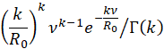 , where Γ is the Gamma function – see Fig. 2A and 2B. With this parameterization of the Gamma distribution, the variance is given by
  . If k≫R0 (formally, k → ∞), each individual has the same individual reproductive number R0. The smaller k, the greater is the variation between individuals. Nevertheless, how many individuals someone infects is still also affected by chance. Let us assume that a person with an individual reproductive number 𝜈 infects a Poisson distributed number of other people (with mean 𝜈), see Fig 2C. Combining this with the Gamma distribution for 𝜈 yields overall a negative binomial distribution for the number of secondary cases j,
  . This distribution is characterized by its mean R0 and the dispersion parameter k. The variance of the negative binomial distribution is given by 𝜎 2= R0 (1 + R0/k). If k is high, k ≫ R0, each infected individual is approximately equally likely to transmit the disease (in the limit k → ∞, each individual has the same “individual basic reproductive number” R0) and all variation comes from randomness in transmission. If k is low, k ≪ R0, there is, in addition to stochasticity in transmission, also the variation between individuals, and the variance is much higher, i.e., some infected individuals transmit the virus to many others (“super-spreaders”), while most infected individuals cause few or no secondary infections. See Fig. 2D for an illustration of how strong this effect can be.
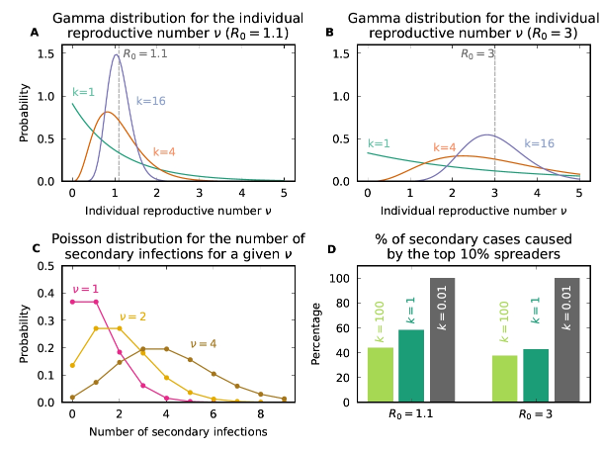
Fig. 2 Dispersion in disease spread. (A) and (B) The average reproductive number is given by R0, but different individuals are more or less likely to transmit the disease (modelled as a Γ-distribution with mean R0 and shape parameter k), which is captured by their individual reproductive numbers 𝜈 and shown here for R0 = 1.1 (A) and R0 = 3 (B). If the shape parameter k is small, the distribution is very broad, and some individuals infect many others, while most infect very few or no others. If the shape parameter k is large, the distribution is centered around R0, but it is broader for larger values of R0. (C) The number of realized secondary infections of an individual is on average given by this individual reproductive number 𝜈 and follows a Poisson distribution with mean 𝜈. Overall, this leads to a negative binomial distribution for the number of secondary cases caused by an individual, which depends on R0 and k (the dispersion parameter of the negative binomial distribution). (D) The fraction of secondary cases caused by the top 10% of all spreaders, which can also be individuals with lower values of 𝜈. This fraction depends strongly on the dispersion parameter k. For large k, almost all individuals spread the infection in the same way, but for small k, the top 10% of spreaders cause virtually all cases (To obtain these values, we first identified the threshold for the top 10% spreaders in the negative binomial distribution,  . Typically, this is not an integer, which was compensated by incorporating only an appropriate fraction of the cases caused by the individual in question. We then averaged the negative binomial distribution from
  to 104 (to approximate ∞), dividing the result by R0 to compare with the average number of secondary cases caused).
Branching processes have a crucial property: they either go extinct or grow to infinity (unless each individual infects exactly one other individual). The outbreak size of an epidemic is, of course, never infinite. At some point, growth slows down since the number of susceptibles becomes limiting. Branching processes do not capture this effect.
2.3 Models with Contact Structure: Network-based Models
Several of the issues arising from the stochastic nature of infections are well described by branching processes. However, on a more fine-grained level, epidemic spread is governed by individuals with possibly overlapping contact structures. Such contact structures can be very different between individuals, and some individuals may be very important for the spread of disease between different communities – while others have a negligible effect. This has led to the development of the field of network epidemiology (Pastor-Satorras and Vespignani 2001, Hufnagel et al. 2004, Salathé et al. 2010), which takes into account the social contact networks of individuals and is concerned with the question of how the structure of these networks will affect the spread of disease. These networks can either be fixed or change over time, which is the case when individuals adjust their ties to the course of an epidemic (Gross et al. 2006, Holme and Saramäki 2012). In addition, it is important to keep in mind that contacts can come with very different risks of infection.
Networks are impressive visualization tools when a local outbreak can be traced back and allow an intuitive approach to understanding how clusters emerge and how they are interconnected. Network science has identified many measures of local network structure and their impact on the overall dynamics within a network (Newman 2010). For example, the identification of central nodes in a network that connect different clusters and their isolation could be very successful in epidemic control – and much more efficient than general contact reduction orders, which affect all individuals in the same way, regardless of their importance for epidemic spread. While this identification of central nodes in infection networks is the basis of contact tracing, contact information is typically not available in the forms of such networks – for privacy reasons and since many health authorities do not use such a perspective and instead treat every case individually and not as part of a network.
Simulating a model of disease epidemics on a contact network show that details of the contact structure can be crucial for the spread of Covid-19 (Firth et al. 2020, Nande et al. 2021). Such simulations can be computationally very costly and they can typically only be done for a limited set of fixed parameters. On the other hand, some fundamental insights about the epidemic spread on networks can already be derived from the network topology alone.
2.4 Complex Agent-based Models
The goal of the epidemiological models discussed above is to illustrate certain aspects of epidemic spread and the dependence of this process on key parameters. This typically requires keeping the number of parameters low to allow analytical insights that are valid beyond a chosen set of numerical parameters (Black and McKane 2012).
A different modeling approach includes as much detail as possible and describes an epidemic based on the behaviors of many individuals and their states in terms of the disease. The rise in computational power in the past decades allowed us to consider more and more sophisticated agents and explore larger and larger systems. In many fields, such large-scale simulations are standard, e.g., in engineering, where the underlying natural laws are known, but the systems are too complex to be understood with any other method. In epidemiology, the underlying laws combine biological and sociological aspects and are thus less clear.
Agent-based approaches for modeling the Covid19 pandemic became popular over the past two years since their results can often be presented in a very intuitive way, and their setup suggests a level of realism that most abstract models cannot reach. Based on extensive simulations, these models take into account various issues such as both the health and economic effects of lockdowns (Silva et al. 2020, Kano et al. 2021). Such models can consider information detailed at the level of single individuals with a complete contact network or full information about testing or vaccination options. For example, drive-in testing options, age-dependent mortality and transmissibility probabilities, and vaccination modes generate a large state-space for the simulated agents to explore (Truszkowska et al. 2021).
Often, such models are valued based on their power to predict the future. This predictive property is of immediate interest during a pandemic, where biological issues interact with social dynamics. The demand for such predictions about the possible course of an epidemic fuels the development of data-driven, complex models. The requirement of quality data to calibrate the models and the assumptions made when the data is unreliable or unavailable make this modeling framework a double-edged sword. If the data and, maybe even more importantly, the remaining underlying assumptions are “good,” then it can be possible to capture the intricacies of social and biological processes that are an integral part of an epidemic. These models are often built around a core very similar to the more basic models discussed above, but they consider additional data such as human mobility patterns, age structure, healthcare capacities, etc. Given the large number of assumptions that arise when such data is integrated, complex models are often a black box that can only be explored by extensive simulations – simple rules of thumb that would lead to general guidelines rarely emerge exclusively from them.
The predictions of complex models have to be interpreted cautiously, and individual forecasts can contain large errors. Comparisons between different forecast models suggest that the best predictions are made when several such models are treated as an ensemble, and their median is taken as a predictor (Friedman et al. 2021, Cramer et al. 2021).
3. Harnessing Models during a Pandemic
3.1 Obtaining Qualitative Insights from Models
3.1.1 Basic Insights from the SIR Model
Several key insights can already be derived from the basic SIR model described above:
– Exponential Dynamics. In the initial phase of an epidemic, we have R(t) ≈ 0 and I(t) ≈ 0. This implies that the number of susceptibles initially stays roughly constant, S(t) ≈ S0 = N. But the number of infected individuals increases rapidly, I(t) ≈ (S0𝛽 − 𝛾) I(t). For S0𝛽 > 𝛾, the number of infected individuals increases exponentially. This is often described by the basic reproductive number R0 = S0 𝛽/𝛾, which corresponds to the average number of infections a single infected person causes in a fully susceptible population. As long as an infected person infects, on average more than one other person, R0 > 1, the number of infected individuals will increase exponentially. Basic reproductive numbers of uncontrolled SARS-CoV-2 have initially been estimated to be 2–4 (Bar-On et al. 2020). Social distancing reduces the number of contacts and thus the rate at which new individuals are infected. This reduction in 𝛽 leads to a lower effective reproductive number Re. Due to governmental regulations and behavioral changes, the effective reproductive number Re has tended to fluctuate around 1 in many countries from mid-2020 to mid-2021 (Arroyo-Marioli et al. 2021).
For S(t)𝛽 < 𝛾, the number of infected individuals decreases exponentially. This situation can be induced by governmental measures and/or behavioral changes. For example, contact restrictions during a lockdown can substantially reduce the number of new infections. In such a phase of exponential decline, the SIR model can help to assess how long a lockdown has to take to reach certain incidence goals, as it suggests a meaningful way to extrapolate.
– Herd Immunity. At which stage does the number of infections decrease again? From Eq. (1b), we can ask when the temporal change of the number of infected individuals starts to decrease, which implies
 I(t) = 0. Setting the right-hand side of Eq. (1b) to 0, we see that this happens when the number of susceptibles is reduced to
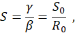 (2)
(2)where we have again used the basic reproductive number R0 – the herd immunity threshold is determined by the inverse of the basic reproductive number. After reaching herd immunity, an infected person will no longer lead to a long infection chain: Initially, when all individuals are susceptible, R0 secondary infections are caused by each infection. However, when only a fraction S(t)/S0 of individuals are susceptible, this is reduced to R0S(t)/S0, which decreases below 1 after herd immunity is reached. Once the fraction of susceptibles is below this threshold, the epidemic subsides.
Without any interventions, herd immunity will eventually be reached via infections. An alternative that became available after only one year in Covid-19 is immunization by vaccination. In the ideal case of a perfect vaccine, one would have to vaccinate a fraction of
 of the population to reach herd immunity – or in other words, reduce the fraction of unvaccinated to values below
  . However, a real vaccine does not work perfectly, and vaccinated individuals are protected from the disease with probability pΕ and can thus still transmit it to others. In this case, the number of secondary cases is given by
 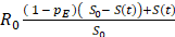 . Thus, we need to reduce the fraction of susceptible, unvaccinated individuals further to values below,
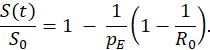 (3)
(3)For the 𝛿-variant, it has been estimated that the Biontech/Pfizer protects individuals against symptomatic disease in 88% of the cases (Lopez Bernal et al. 2021). For simplicity, let us assume that this is also the probability to protect against transmission. For R0 = 5, a current estimate for the 𝛿-variant (Liu and Rocklöv 2021), we would reach herd immunity by vaccination only when the fraction of vaccinated reaches
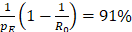 . For an R0 >
  , herd immunity with a vaccine that protects against transmission with probability
  would not be feasible anymore, even if we optimistically assume that there is no waning of protection with time. Moreover, vaccinated individuals are still getting infected in this scenario. However, there is still a considerable individual and societal benefit from vaccines in such a situation: Typically, vaccines offer a good protection against severe disease and thus avoid overloading the public health system. In addition, the partial protection by vaccination contributes to a less severe epidemic.
 – Vaccination vs. natural immunity. By vaccination, people turn from susceptible into a state that – in the context of this model – is equivalent to those recovered from the disease. Thus, we can expect that once the herd immunity threshold is reached by vaccination, infection chains are short, and the epidemic is effectively controlled such that not many new infections can occur after this point.
However, this is not true for naturally acquired immunity occurring in an uncontrolled epidemic. In this case, many infectious individuals are present at the stage when herd immunity is reached. This peak in the fraction of infected individuals is given by (see Appendix A or Eq. (2.4) in (Brauer 2008))
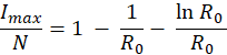 (4)
(4)These infectious individuals will still infect many others and cause additional infections and additional deaths. Stopping the pandemic by a precisely targeted vaccination campaign shortly before herd immunity is reached seems a possibility, but it seems a very theoretical one that is unrealistic in any real scenario. Nevertheless, mitigation measures and behavioral changes slow the course of a pandemic such that the overshoot – the difference between the total number of cases at the end of the pandemic and the herd immunity threshold – is smaller than in an uncontrolled pandemic.
In the SIR model, which assumes a homogeneous population, the herd immunity threshold is the same irrespective of whether it is infection-induced or vaccination-induced. This is usually not true in a heterogeneous population with a complex population structure. Since disease spread is affected by heterogeneity (e.g., highly connected individuals are more likely both to be infected and to infect others), the infection-induced herd immunity threshold in a heterogeneous population differs from that in a homogeneous population and from the one corresponding to random vaccination of individuals (Ferrari et al. 2006, Fine et al. 2011, Britton et al. 2020, Ellison 2020). Targeted non-random vaccination may be used to reduce the number of people that need to be immunized to reach herd immunity in a heterogeneous population. However, this may oppose other goals of vaccination, especially the protection of the vulnerable risk groups.
3.1.2 Assessing Outbreak Probabilities with Branching Processes
Not every infection introduced into an area seeds an infection chain that leads to a considerable number of cases – an event often referred to as an “outbreak” that can only be stopped by interventions and would otherwise continue to spread. Only a few infection events may occur before the process goes extinct due to stochastic fluctuations. How likely is it that a primary case launches a large outbreak? This is an important factor in making risk assessments during a pandemic, and answering this question is a classical application of branching process theory. For example, branching processes have been applied to estimate the probability that an introduced case would cause a large outbreak (Kucharski et al. 2020) or to assess the impact of different mitigation measures to contain an outbreak (Levesque et al. 2021).
Let us denote the outbreak probability by Poutbreak. It is easier to consider the complementary probability  , i.e., the probability that the process goes extinct. Suppose the primary case causes j secondary infections (which happens with probability pj). In that case, the process goes extinct if none of these j new cases launches an outbreak. According to the definition of branching processes, these j processes develop independently from each other. Therefore, we have
 (5)
(5)
which can be solved to obtain the outbreak probability, if the distribution of secondary cases {pj} is known. The outbreak probability is zero if R0 ≤ 1 (unless p1 = 1). It is larger than zero if R0 > 1.
It is possible to derive an approximation if the mean number of secondary cases R0 is just slightly larger than 1,
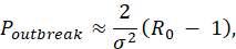 (6)
(6)
where 𝜎2 is the variance of the distribution (see Equation 14.69 in Otto and Day 2007). From this approximation, we can gain an important insight (which also holds for large R0): For a given R0, the outbreak probability is lower if the variance in the number of secondary infections is larger. This means that the outbreak probability is lower when few individuals are responsible for most infections and the majority of individuals infect only a few others or none at all, compared to a situation in which all patients infect roughly the same number of individuals. However, if an outbreak happens, it can be explosive. Importantly, this insight relates to the distribution of secondary cases and not to the distribution of contacts that an individual has in a network. A network with greater heterogeneity in contacts (but equal mean number of contacts) does not necessarily imply a lower outbreak probability (Alexander and Day 2010). The difference is because an individual with more contacts is also more likely to become infected, i.e., the infected individuals are not a random subset of the total population. In the same way, branching processes cannot only be used to assess the outbreak probability of local (or global) epidemics, but also new viral variants.
Importantly, the outbreak probability of a branching process is the probability that it grows to infinity, and the extinction probability is the probability that it does not do so. However, ultimate extinction does not mean that there cannot be many cases. In fact, even if R0 < 1 (and hence Poutbreak = 0), the outbreak size can be substantial (see e.g. the simulation for the spread of Ebola in Althaus 2015). However, this captures the real behaviour of disease spread. In more complex models in which growth of the epidemic is limited, and the number of cases decreases at some point due to herd immunity, the distribution of outbreak sizes is bimodal if R0 > 1: it has one peak at rather low values (but the tail of this peak can reach into substantial outbreak sizes) and another one at very high outbreak sizes. These peaks correspond to the two outcomes – extinction or infinite growth – of the branching process. For R0 ≤ 1, the distribution is unimodal, and the peak is at low outbreak sizes. Again, such an outbreak can extend to considerable sizes.
3.1.3 Contact Tracing in Network and Other Models
Individuals are embedded in various overlapping social networks such as schools, work, friends, etc. When an epidemic arises, breaking the chain of transmission is critical. Ideally, when a focal individual is found to be infected, all contact persons who had potentially infectious contact with the focal are identified and informed. Contact tracing needs to be fast and efficient to keep up with the transmission speed. Thus, the process is the most effective when done very fast or in a slowly spreading epidemic (Fraser et al. 2004).
Hethcote et al. (1982) were among the first to assess the effectiveness of contact tracing in controlling disease spread – in this case Gonorrhoea – by mathematical modeling (see also Chapter 6 in Hethcote and Yorke (1984) and the highlighting article by May (1981)). They already consider two ways of contact tracing – forward and backward tracing,
- – (i) Trace to whom the focal individual has potentially already spread the disease (forward tracing) or
- – (ii) Trace from whom the individual has been infected in the first place (backward tracing)?
While forward tracing intuitively appears like the more natural way to interrupt infection chains, and backward tracing appears to be more relevant in a context that aims to look into history, it has been shown that backward tracing can be remarkably efficient due to the heterogeneity of contact networks (cf. also the findings in the early study by Hethcote et al. 1982). In any real social contact network, some individuals are more connected than others. As also diseases are transmitted via these contacts, highly connected individuals are more likely to be infected, and these individuals could turn into super-spreaders. To identify those super-spreaders, the fact that the contacts of any focal individual (i.e., the infected individual whose contacts are being traced) tend to have more contacts than the focal individual itself can be exploited via backward tracing (Kojaku et al. 2021). Once such super-spreaders are identified, their contacts have to be informed – formally leading to a combination of backward and forward tracing.
There are a variety of ways to model explicit contact structures. Hethcote et al. (1982) divide the population into several groups, based among other criteria on their number of contacts. At a more detailed level, individual-based models implementing contact structures have been used in a variety of infectious diseases such as smallpox (Porco et al. 2004), tuberculosis (Kasaie et al. 2014), and others, and such models have also been applied to model contact tracing of Covid-19 where e.g. the dynamics in an epidemiological model has been simulated and visualised on (pre-Covid-19) real world social networks (Firth et al. 2020). Such detailed models often do not allow for a precise understanding of the processes. Pair approximation (Eames and Keeling 2002, Clarke et al. 2012, Bradshaw et al. 2021, Endo et al. 2021, Müller and Hösel 2020, Fyles et al. 2021) is one way of recovering some analytical tractability in these complex models while accounting for certain elements of the contact structure (such as the probability that a neighbour of an infected individual is also infected or the inclusion of tracing probability/delay) (Barlow 2020). Aspects of contact tracing can also be analyzed by branching processes. By allowing to study at least part of the problem analytically, branching process approaches can highlight key parameters and their role in contact tracing. For example, when the delay between the first transmission and isolation is too long or when there are too many asymptomatic cases, the efficiency of tracing is very limited (Hellewell et al. 2020).
Contact tracing requires a lot of resources and thus tends to be slow if done manually. In principle, it can be greatly enhanced when the relevant information is automatically made available, e.g., via proximity data from mobile phones or warning apps. Some countries have enforced this rigorous contact tracing and have been very efficient in containing the epidemics with this approach (Ryan 2020). However, due to concerns about sharing this data with companies or governments, many countries have implemented digital contact tracing on a voluntary basis (and in some cases also without central data storage). In this case, it is important to reach a sufficient number of individuals to make this approach successful (Juneau et al. 2020). Mathematical considerations based on the topology of the contact network or on the parameters of the tracing strategies can help to optimize this approach and to assess its benefits.
3.2 Data Interpretation
3.2.1 Estimating the Effect of Control Measures
The SIR model has been used early in the pandemic to fit the temporal development of new infections to assess the impact of mitigation measures. In retrospect, one can then argue at which point the increase in the number of new infections has changed or even stopped – and put this into context with the political measures valid at that time (Dehning et al. 2020). However, such an approach is based on the assumption that changes in case numbers are directly caused by mitigation measures, which may not always be accurate. E.g., a correlation between seasonality and certain measures could be misinterpreted as a successful mitigation measure. Later in 2020, data on mitigation measures were collected across many countries, which allowed to disentangle the impact of measures introduced at the same time (Brauner et al. 2021, Haug et al. 2020). Also, these studies have to be taken with a grain of salt, as similar measures may have very different consequences in different countries. However, some general pictures emerge, e.g., the closing of non-essential businesses was found to be less efficient than the closing of schools (which tends to reduce many contacts indirectly, see Litvinova et al. 2019 for a study in the context of influenza). This could, for example happen because parents stay at home to take care of their children. However, the role of school closures on epidemic spreading remains a subject of current research (Fukumoto et al. 2021).
3.2.2 Estimating Heterogeneity in Transmission
For the dynamics of the epidemic and the choice of mitigation interventions, it is important to know whether super-spreader events drive an epidemic or if all individuals can be considered to be approximately equal. Ideally, we have data from contact tracing that tells us for a reasonably large number of individuals how many others they infected. In that case, we would have an empiric distribution of secondary cases. Assuming a negative binomial distribution, the mean R0 and the dispersion parameter k can then be obtained from this data, e.g., by maximum likelihood estimation (Lloyd-Smith et al. 2005, Althaus 2015).
Such data were unavailable in the very early phase of the Covid-19 pandemic. There were total case counts, but even those were not reliable. Nevertheless, to obtain at least some estimate already in January 2020, Riou and Althaus (2020) simulated epidemic outbreaks as branching processes with negative binomially distributed secondary cases for a range of values of R0 and k, varying other parameters such as the time of the first case as well. From comparing a large number of such simulated epidemics to the observed case numbers (accounting for large uncertainty), they estimated R0 (median value of 2.2) and k (median value of 0.54). Given the scarcity of the data and the uncertainty in many parameters, such as the timing of the pandemic’s start, these estimates are subject to much uncertainty, and a large range of k values can explain the observed data.
Almost simultaneously to the simulation study by Riou and Althaus (2020), data on the number of secondary cases caused by index cases became available. For example, Bi et al. (2020) used data from detected cases between January 14 to February 9 to estimate k to be 0.54 and Re to be 0.4 in Shenzhen, China. Based on contact tracing data collected in France between January 24 and March 30, 2020, Paireau et al. (2020) estimated k to be 0.17 and Re to be 0.3 (or k = 0.28 and Re = 0.9, if retrospectively reconstructed transmission events were taken into account). These estimates are quite different from one another. It should be clear that (besides uncertainty in the estimates), there is no universally true k, since it depends, for example, on the structure of the society and the effects of current mitigation measures in that society.
To put these estimates for the dispersion parameter in some context, the estimate by Lloyd-Smith et al. (2005) for a SARS outbreak in Singapore was k = 0.16 with an Re value of 1.63 (i.e., highly overdispersed), while (using a different model) k was estimated to be 0.94 and Re to be 1.38 for the 1918 influenza pandemic in Baltimore (Fraser et al. 2011). All these estimates show that heterogeneity in transmission is a rule rather than the exception in infectious diseases – some people are much more likely to spread the disease than others.
3.2.3 Short-term Extrapolation
In the short run and in situations well below the herd immunity threshold, the SIR model predicts either exponential growth (S(t) 𝛽 > 𝛾) or exponential decrease of infections (S(t) 𝛽 < 𝛾). This exponential dynamics can be used to extrapolate the dynamics for short time intervals. For example, it gives an idea about the necessary duration of a lockdown until certain incidence targets are reached – assuming that nothing else would change. In times of increasing case numbers, this approach allows to assess how fast case numbers reach a level that can no longer be controlled, e.g., by contact tracing through health authorities, and thus how fast political decisions need to be made to avoid this.
However, these extrapolations are blind towards additional issues that come up and can drive the course of an epidemic: New restrictions or taking back restrictions only have an effect after a delay. Upcoming vacation periods or holidays may change the disease dynamics, and weather changes can drive social behavior. In addition, novel mutations can change the biology of a virus and render such extrapolations irrelevant. Thus, these extrapolations only make sense in the short term and even then break down if the factors affecting the incidence are not constant during the fit and extrapolation windows. They help to get an intuition of the current situation but do not predict the future and must be handled with care.
As an example, Fig. 3 shows extrapolations of the incidences in several German states in early May 2021.
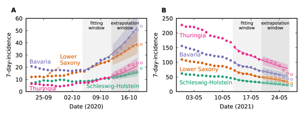
Fig. 3 Short-term extrapolation of the incidences for the federal states of Germany in (A) autumn 2020 and (B) spring 2021. The filled symbols are 7-day incidence values, i.e., the number of new cases within a week per 100000 people. The short-term extrapolation used the data from fitting the function f (t) = a bt to the fitting window, i.e. a and b were estimated by minimizing the sum of squared residual errors in the fit window. We used the variance of these estimated parameters to calculate the confidence interval. Subsequently, these parameters were used to extrapolate into the immediate future. The real incidences that occurred in the extrapolation window (and beyond) are shown as open symbols. Using the inverse of the exponential function  , the time 𝜏 to a future incidence value x can be estimated. For example, in (A), such an estimate could be used to assess at which time the incidences call for further interventions. In (B), one could use the same approach to estimate when certain restrictions can be lifted again. The COVID19 dataset for Germany is publicly available and can be downloaded from the RKI data repository (Robert-Koch-Institute, 2021a), last accessed June 21, 2021.
3.3 Making Predictions
3.3.1 Predictions based on Additional Knowledge
Data-driven models for the Covid-19 pandemic are typically based on the available data since early 2020. However, they typically do not take into account some known properties of coronaviruses. One such property known for other coronaviruses is seasonality in the virus transmission. At the start of the current pandemic, this seasonality was not yet visible in the data for SARS-Cov-2 and was thus initially not taken into account by data driven models. Do we need to work with sophisticated models to assess the impact of such seasonality? It turns out that it can be enough to work with a time-dependent infection parameter 𝛽, which can be described by a sine wave with a period of one year. A minimal model based on this idea was published in mid-March 2020. The authors made it very clear that their model does not qualify as a prediction but as an exploration of different scenarios (Neher et al. 2020). Nonetheless, they found that “Simulations of different scenarios show that plausible parameters result in a small peak in early 2020 in temperate regions of the Northern Hemisphere and a larger peak in winter 2020/2021”. In reality, many additional factors affected the course of the pandemic. However, even a very simple model with few parameters illustrated a scenario that unfortunately became true.
3.3.2 Assessing Consequences of Virus Evolution
Another point where predictions are not possible based on infection numbers alone is the future spread of new variants. If we only look at the total number of cases, we cannot see any dynamics on the level of virus strains. But new variants could increase in absolute numbers, while old variants are dominating the dynamics and lead to an overall decreasing trend. In the simplest case, the dynamics can be described by the sum of an exponentially increasing and an exponentially decreasing function,
 (7)
(7)
where Iold(0) and Inew(0) are the number of infected individuals carrying the old and the new variant at the initial time t = 0 and bold and bnew are the factors with which they increase or decrease. The first summand reflects the dynamics of the old variant and with bold < 1 it decreases. The second sum gives the dynamics for the new variant and with bnew > 1 it increases. As long as the new variant is rare, the first summand dominates the behavior, such that the total number of cases decreases. However, once the new variant becomes frequent, the second summand becomes important, and the number of cases rebounds. Overall, this results in a U-shaped curve (Fig. 4A).
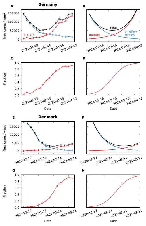
Fig. 4 Modelling the take-over of a new variant. Early in 2020, the mutant variant B.1.1.7 (“𝛼-variant”) became dominant in many European countries during a time where the general incidences were decreasing. The dynamics can be well described by a sum of two exponential functions, an increasing one describing the new variant and a decreasing one describing all other strains. Here, we show the dynamics for Germany (panels A–D) and Denmark (panels E–H). The data is given in terms of weeks, and we plot the weekly data point on the date of the Monday of the corresponding week. We fitted the absolute number of wild-type and mutant cases (obtained from extrapolating the fraction of this variant found in genomic data) during the initial phase (filled symbols in panels A and E) to exponential functions. Panels B and F show the fitted exponential functions as well as the total number of cases given by their sum. From the data itself, we calculated the fraction of infections caused by the mutant (panels C and G). The qualitative agreement with the fractions calculated from the fits (panels D and H) is very good. Based on this simple approach, in Germany it was possible to estimate that the vast majority of cases are caused by the mutant almost two months ahead of time. Data for Germany from the reports on variants of concern by the Robert Koch Institute, (Robert-Koch-Institute, 2021b), last accessed June 21, 2021, data for Denmark from (Danish Covid-19 Genome Consortium, 2021), last accessed on June 21, 2021.
This combination of a variant increasing exponentially, while the prevalent variant was decreasing exponentially, was observed in many European countries in January – March 2021. As an example, Fig. 4A/B and 4E/F show the developments in Germany and Denmark (where more detailed data on new variants was available) between the end of December 2020 and mid-April 2021. In Denmark, the exponential trend in the case numbers caused by the B.1.1.7 variant eventually did not continue; instead, case numbers started to plateau. In Germany, the exponential trend in the case numbers caused by the B.1.1.7 variant eventually led to a new epidemic wave in March and April 2021.
It should be clear that as for the extrapolations discussed above, fitting two exponential functions on the numbers of two different variants does not allow us to make accurate quantitative predictions for the future either, especially not beyond a small time window. E.g., as mentioned above, exponential growth eventually stopped in Denmark. However, looking at case numbers in that way prevents being deceived by overall declining cases, and making exponential fits can help to gain a quick grasp of the new variant’s risk and estimate when the trend in the development of the case numbers will reverse.
Media often report the relative frequencies of variants of concern. In the model in Eq. (7), the relative frequency pnew(t) of the new variant is given by
 (8)
(8)
see Fig. 4C/D and 4G/H. The speed of increase of the relative frequency of a variant describes how much easier it spreads. However, it gives no direct insights into the risk posed by the new variant, since one cannot directly see whether the new variant is under control or not, as long as overall case numbers are declining. For this, considering absolute numbers is more suitable.
3.3.3 Long-term Predictions
What do mathematical models tell us about the long-term dynamics of such a pandemic? The key parameters of these models depend on the transmission dynamics, which can be driven by behavioral changes as a response to the introduction or relaxation of governmental responses during a pandemic and seasonal effects. But a further crucial factor is the immune response to infections and vaccination. It is particularly important how well individuals are protected from current and future strains and how long this protection will last. Mathematical and computational models allow exploring wide parameter ranges that explore scenarios ranging from complete elimination of the virus to the transition to an endemicity (Saad-Roy et al. 2020). Taking into account the age structure of the population and differences in the adaptive immune system between children and adults, some of these models predict that in the long run, we will reach an endemic state where most primary cases occur in young children (Lavine et al. 2021). It should be noted that such predictions crucially depend on the features of immunity and much less on the current number of infected cases as described, e.g., by the SIR model.
However, on a time scale of weeks or months, it is important to assess whether we reach a peak of an epidemic wave or not. Even in the absence of further complications such as vaccination campaigns, such an assessment is surprisingly difficult – and due to the stochastic nature of the disease dynamics more data is necessary, but not sufficient to make realistic predictions (Castro et al. 2020). The end of the epidemic remains unclear.
3.3.3 Long-term Predictions
What do mathematical models tell us about the long-term dynamics of such a pandemic? The key parameters of these models depend on the transmission dynamics, which can be driven by behavioral changes as a response to the introduction or relaxation of governmental responses during a pandemic and seasonal effects. But a further crucial factor is the immune response to infections and vaccination. It is particularly important how well individuals are protected from current and future strains and how long this protection will last. Mathematical and computational models allow exploring wide parameter ranges that explore scenarios ranging from complete elimination of the virus to the transition to an endemicity (Saad-Roy et al. 2020). Taking into account the age structure of the population and differences in the adaptive immune system between children and adults, some of these models predict that in the long run, we will reach an endemic state where most primary cases occur in young children (Lavine et al. 2021). It should be noted that such predictions crucially depend on the features of immunity and much less on the current number of infected cases as described, e.g., by the SIR model.
However, on a time scale of weeks or months, it is important to assess whether we reach a peak of an epidemic wave or not. Even in the absence of further complications such as vaccination campaigns, such an assessment is surprisingly difficult – and due to the stochastic nature of the disease dynamics more data is necessary, but not sufficient to make realistic predictions (Castro et al. 2020). The end of the epidemic remains unclear.
4. Discussion
Here, we have discussed some of the most basic models for the dynamics of an epidemic. These models can explain many important aspects, such as the dependence of the herd immunity threshold on the basic reproductive number of an epidemic or the importance of heterogeneity in the spread of infectious diseases. However, they are sketches of an epidemic, and in reality, the dynamics are a complex conglomeration between the effects arising from many aspects that are not included in these models, e.g., spatial population structure, human mobility patterns, feedbacks between behavior and the state of the epidemic, and many others. In addition, more complicated models may consider economic aspects, different social groups, age effects, etc. Whether the inclusion of as many aspects of reality as possible is desirable is answered differently in the different scientific communities, where also the typical modeling setups differ. Scientists from diverse fields have contributed to models of the Covid-19 pandemics and addressed them in ways that build on the paradigms of their fields: Physicists like to point out and exploit connections on a general, abstract level, which, e.g., leads to epidemiological models based on dynamic density functional theory from soft matter physics (Te Vrugt et al. 2020). Network scientists stress the importance of contact networks and aim to describe aspects arising from these structures (Nande et al. 2021, Kojaku et al. 2021). The machine learning community focuses on the large datasets available in the pandemic and forecasts the future course based on these datasets and less on mechanistic aspects. Engineers who are used to massive simulation models tend to develop more complex mechanistic models that ideally serve to make realistic predictions (Müller et al. 2021). While these models are developed and communicated in different ways, they involve a core driven by epidemiological considerations. Thus, they are naturally connected to the established models developed by theoretical epidemiologists, who have also not only applied their existing models, but also adjusted and extended them to address the specificities of Covid-19.
So which models are the best ones? The choice of the model depends heavily on the actual purpose of the models. Is our aim a precise prediction of a system? And if so, along which time scales? Or is our aim to have a more detailed understanding of the processes underlying epidemic spread? Or do we use them to illustrate an important point, such as the importance of super-spreading? If we are only interested in making short term predictions, an extrapolation of current trends may be sufficient. But predictions over several weeks may already require a different approach: For example, when the virus variant B.1.1.7 (𝛼-variant) was first spreading across Germany and Denmark, someone modeling the course of the epidemics based only on knowledge of the total case numbers would have concluded that case numbers should continue to go down. But as the simple model of two exponential functions explained above shows, the knowledge about the abundance of the virus variant allowed to give an early warning to what would be coming. For long-term predictions, completely different aspects, e.g., arising from yet unknown virus evolution and the long-term dynamics of the immune system after infection or vaccination, have to be considered. If we are instead interested in the processes underlying epidemic spread, we must instead develop models where the impact of parameters can be analysed in more detail. These are exactly the kind of models we put into our focus. These models aim to give quantitative insight and assess the impact of specific control measures on a more abstract level. At the same time, these simple models can help in data interpretation and also in making first extrapolations given the immediate past.
At least in retrospect, one could argue that the quality of models can be assessed: Given past disease trajectories, which ones are best described by a certain model? This only makes sense for models that make concrete predictions. However, as soon as these models are communicated to the public or even used to facilitate political decision-making, they interfere with their own predictions: If a model predicts that the pandemic situation will improve rapidly, people may adjust their behavior such that the situation escalates again. If a model predicts that case numbers rise rapidly, politicians may be inclined to take more extreme countermeasures. Thus, even in retrospect, it is challenging to assess the model’s predictive ability.
More complex models are typically more challenging to handle. They have to be sufficiently robust, as they can only be analyzed based on large-scale simulations. Usually, the parameter space is so large that such robustness checks are computationally challenging, and a full exploration of the relevant parameter range may even be impossible. In addition, one has to assess the structural stability, i.e., if the choices made for functional dependencies can be varied without changing the general result. Moreover, in the application of such models one needs to keep in mind that the quality of the prediction is typically evaluated in terms of past data. The firm establishment of causal links, e.g., between control measures and new infections, remain elusive, as controlled experiments are not feasible in the context of an epidemic. However, such models are very useful if interpreted in the proper context, as they allow exploring various scenarios for the further development of an epidemic.
A separate point is that how models in science are developed is very different from the development of applied software. Mathematical models in the sciences are often developed, extended, or corrected over long time scales and published in peer-reviewed journals. The focus is on the insight arising from the model, and often, many different implementations are available, with analytical approaches complementing simulations. In contrast, commercial software development focuses on a single implementation. Especially where security is crucial (such as railway systems or autonomous vehicles), such software has to be developed under a much more rigorous code testing regime than exploratory scientific models. Since many models developed to understand the course of the Covid-19 pandemics are immediately discussed by the media, and by the public, such a more rigorous testing regime would also be desirable when scientific computational models are finding immediate applications. But in situations where time pressure is as high as in a pandemic, it would be challenging to implement such a regime.
If mathematical and computational models become important to help decision-makers steer entire countries through a pandemic, these models must be accurate and fit this purpose. If one would make all decisions dependent on predictions of a single, complex model, can we as an entire society fully rely on its accuracy? Despite the laudable availability of the source code of these models, which is now standard, it is not easy to take these models apart: To understand the details of the code and the influence of its assumptions, it needs true experts, and for most other people, such models remain black boxes. The basic models we focus on here are accessible to anyone willing to engage in quantitative thinking. Thus, they are more transparent than many models based purely on simulation. These basic models provide simple rules of thumb that do not make more complex models superfluous but can help understand if a complex model’s output can make sense. More importantly, basic models can be the first guides on how to assess the situation, and they allow to analyze important issues, such as the impact of super-spreading, in a rigorous and fully transparent way.
In the past two years, we have seen how powerful different kinds of mathematical models can be. Mathematical models have played a pivotal role in helping us understand the dynamics of the pandemic, in guiding our intuition, in making sense of data, and in predicting the consequences of disease spread, viral evolution, and mitigation measures. We hope that this contributes to an increased appreciation of the value of mathematical modeling and the realization that mathematical biology is not an abstract science without a connection to reality or benefit to society, but fundamental for our understanding of the biological processes around us. We hope that also hiring committees will recognize that expertise in this field is urgently needed within the biological sciences, medicine, and public health.
A Maximal Number of Infected Individuals
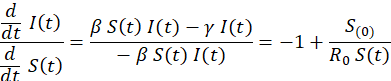
When the infection curve reaches its maximum, we have  in Eq. (1b). This implies that the number of susceptible individuals at this point is given by . We can use Eqs. (1a) and (1b) to switch to a description of curves in the (S, I) plane. In this way, we find
 (9)
(9)
or  . Integration leads to
 (10)
(10)
or
 (11)
(11)
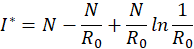
Since we have S (0) ≈ N and I (0) ≈ 0, we can calculate the maximum  from
from  ,
,
 (12)
(12)
which, renaming  = Imax, corresponds to Eq. (4).
References
Alexander, H. K., and Day, T.: Risk factors for the evolutionary emergence of pathogens. Journal of the Royal Society Interface 7/51, 1455–1474 (2010). doi:10.1098/rsif.2010.0123
Althaus, C. L.: Ebola superspreading. The Lancet Infectious Diseases 15/5, 507–508 (2015)
Arroyo-Marioli, F., Bullano, F., Kucinskas, S., and Rondón-Moreno, C.: Tracking of Covid-19: A new real-time estimation using the Kalman filter. PLoS One 16/1, e0244474 (2021)
Bar-On, Y. M., Flamholz, A., Phillips, R., and Milo, R.: Science forum: SARS-CoV-2 (Covid-19) by the numbers. Elife 9, e57309 (2020)
Barlow, M. T.: A branching process with contact tracing. arXiv:2007.16182 (2020)
Bernoulli, D.: Essai d’une nouvelle analyse de la mortalité causée par la petite vérole et des advantages de l’inoculation pour la prévenir. Mém. Math. Phys. Acad. Roy. Sci., Paris 1–45 (1766)
Bernoulli, D., and Blower, S.: An attempt at a new analysis of the mortality caused by smallpox and of the advantages of inoculation to prevent it. Reviews in Medical Virology 14, 275–288 (2004)
Bi, Q., Wu, Y., Mei, S., Ye, C., Zou, X., Zhang, Z., Liu, X., Wei, L., Truelove, S. A., Zhang, T., Gao, W., Cheng, C., Tang, X., Wu, X., Wu, X., Sun, B. Y., Huang, S., Sun, Y., Zhang, J., Ma, T., Lessler, J., and Feng, T.: Epidemiology and transmission of Covid-19 in 391 cases and 1286 of their close contacts in Shenzhen, China: a retrospective cohort study. Lancet Infect Dis 20, 911–19 (2020)
Black, A. J., and McKane, A. J.: Stochastic formulation of ecological models and their applications. Trends in Ecology and Evolution 27/6, 337–345 (2012). doi:10.1016/j.tree.2012.01.014
Bradshaw, W. J., Alley, E. C., Huggins, J. H., Lloyd, A. L., and Esvelt, K. M.: Bidirectional contact tracing could dramatically improve Covid-19 control. Nature Communications 12/232 (2021). doi:10.1038/s41467-020-20325-7
Brauer, F.: Compartmental Models in Epidemiology; pp. 19–79. Berlin, Heidelberg: Springer (2008). doi:10.1007/978-3-540-78911-6_2
Brauner, J. M., Mindermann, S., Sharma, M., et al.: Inferring the effectiveness of government interventions against Covid-19. Science 371/6531 (2021)
Britton, T., Ball, F., and Trapman, P.: A mathematical model reveals the influence of population heterogeneity on herd immunity to SARS-CoV-2. Science 369/6505, 846–849 (2020). doi:10.1126/science.abc6810
Castro, M., Ares, S., Cuesta, J. A., and Manrubia, S.: The turning point and end of an expanding epidemic cannot be precisely forecast. Proc Natl Acad Sci 117/42, 26190–26196 (2020)
Clarke, J., White, K. A. J., and Turner, K.: Exploring Short-term responses to changes in the control strategy for Chlamydia trachomatis. Computational and Mathematical Methods in Medicine 2012/803097 (2012). doi:10.1155/2012/803097
Cramer, E. Y., Lopez, V. K., Niemi, J., et al.: Evaluation of individual and ensemble probabilistic forecasts of Covid-19 mortality in the US. medRxiv (2021). doi:10.1101/2021.02.03.21250974
Danish Covid-19 Genome Consortium: (2021) Available at: https://www.covid19genomics.dk/statistics
Dehning, J., Zierenberg, J., Spitzner, F. P., Wibral, M., Neto, J. P., Wilczek, M., and Priesemann, V.: Inferring change points in the spread of Covid-19 reveals the effectiveness of interventions. Science 369/6500 (2020)
Eames, K. T. D., and Keeling, M. J.: Modeling dynamic and network heterogeneities in the spread of sexually transmitted diseases. Proc Natl Acad Sci 99/20, 13330–13335 (2002). doi:10.1073/pnas.202244299
Ellison, G.: Implications of heterogeneous SIR models for analyses of Covid-19. Working Paper 27373, National Bureau of Economic Research (2020)
Endo, A., Centre for the Mathematical Modelling of Infectious Diseases Covid-19 Working Group, Leclerc, Q. J., et al.: Implication of backward contact tracing in the presence of overdispersed transmission in Covid-19 outbreaks. Wellcome Open Research 5/239 (2021). doi:10.12688/wellcomeopenres.16344.3
Ferrari, M. J., Bansal, S., Meyers, L. A., and Bjørnstad, O. N.: Network frailty and the geometry of herd immunity. Proceedings of the Royal Society B: Biological Sciences 273/1602, 2743–2748 (2006)
Fine, P., Eames, K., and Heymann, D. L.: Herd immunity: A rough guide. Clinical Infectious Diseases52/7, 911–916 (2011)
Firth, J. A., Hellewell, J., Klepac, P., Kissler, S., Kucharski, A. J., and Spurgin, L. G.: Using a real-world network to model localized Covid-19 control strategies. Nature Medicine 26/10, 1616–1622 (2020). doi:10.1038/s41591-020-1036-8
Fraser, C., Riley, S., Anderson, R. M., and Ferguson, N. M.: Factors that make an infectious disease outbreak controllable. Proc Natl Acad Sci USA 101/16, 6146–6151 (2004). doi:10.1073/pnas.0307506101
Fraser, C., Cummings, D. A. T., Klinkenberg, D., Burke, D. S., and Ferguson, N. M.: Influenza transmission in households during the 1918 pandemic. Am J Epidemiol 174/5, 505–514 (2011). doi:10.1093/aje/kwr122
Friedman, J., Liu, P., Troeger, C. E., et al.: Predictive performance of international Covid-19 mortality forecasting models. Nature Communications 12/1, 1–13 (2021)
Fukumoto, K., McClean, C. T., and Nakagawa, K.: No causal effect of school closures in Japan on the spread of Covid-19 in spring 2020. Nature Medicine 27/12, 2111–2119 (2021)
Fyles, M., Fearon, E., Overton, C., University of Manchester Covid-19 Working Group, Wingfield, T., Medley, G. F., Hall, I., Pellis, L., and House, T.: Using a household structured branching process to analyse contact tracing in the SARS-CoV-2 pandemic. medRxiv 2021. doi:10.1101/2021.02.03.21250992
Gog, J. R.: How you can help with Covid-19 modelling. Nature Reviews Physics 2/6, 274–275 (2020)
Gross, T., Dommar D’Lima, C. J., and Blasius, B.: Epidemic dynamics on an adaptive network. Phys Rev Lett96/208701 (2006)
Hamer, W. H.: The Milroy Lectures on Epidemic Disease in England – The Evidence of Variability and Persistence of Type. Lancet 1, 733–739 (1906)
Haug, N., Geyrhofer, L., Londei, A., Dervic, E., Desvars-Larrive, A., Loreto, V., Pinior, B., Thurner, S., and Klimek, P.: Ranking the effectiveness of worldwide Covid-19 government interventions. Nature Human Behaviour 4/12 1303–1312 (2020)
Hellewell, J., Abbott, S., Gimma, A., et al.: Feasibility of controlling Covid-19 outbreaks by isolation of cases and contacts. The Lancet Global Health8/4, e488–e496 (2020)
Hethcote, H. W., and Yorke, J. A.: Gonorrhea transmission dynamics and control. Lecture Notes in Biomathematics 56 (1984). doi:10.1007/978-3-662-07544-9
Hethcote, H. W., Yorke, J. A., and Nold, A.: Gonorrhea modeling: a comparison of control methods. Mathematical Biosciences 58/1, 93–109 (1982). doi:10.1016/0025-5564(82)90053-0
Holmdahl, I., and Buckee, C.: Wrong but useful – what covid-19 epidemiologic models can and cannot tell us. New England Journal of Medicine 383, 303–305 (2020). doi:10.1056/NEJMp2016822
Holme, P., and Saramäki, J.: Temporal networks. Physics Reports 519/3, 97–125 (2012)
Hufnagel, L., Brockmann, D., and Geisel, T.: Forecast and control of epidemics in a globalized world. Proc Natl Acad Sci 101/42, 15124–15129 (2004)
Juneau, C.-E., Briand, A.-S., Pueyo, T., Collazzo, P., and Potvin, L.: Effective contact tracing for Covid-19: A systematic review. medRxiv (2020)
Kano, T. Yasui, K., Mikami, T., Asally, M., and Ishiguro, A.: An agent-based model of the interrelation between the Covid-19 outbreak and economic activities. Proceedings of the Royal Society A, 477/2245, 20200604 (2021). doi:10.1098/rspa.2020.0604
Kasaie, P., Andrews, J. R., Kelton, W. D., and Dowdy, D. W.: Timing of Tuberculosis Transmission and the Impact of Household Contact Tracing. An Agent-based Simulation Model. Am J Respir Crit Care Med 189/7, 845–852 (2014).
doi:10.1164/rccm.201310-1846oc
Kermack, W. O., and McKendrick, A. G.: A contribution to the mathematical theory of epidemics. Proceedings of the Royal Society B, 115, 700–721 (1927)
Kojaku, S., Hébert-Dufresne, L., Mones, E., Lehmann, S., and Ahn, Y.-Y.: The effectiveness of backward contact tracing in networks. Nature Physics 17, 652–658 (2021)
Kucharski, A. J., Russell, T. W., Diamond, C. et al.: Early dynamics of transmission and control of Covid-19: a mathematical modelling study. Lancet Infect Dis 20/5, 553–558 (2020). doi:10.1016/S1473-3099(20)30144-4
Lavine, J. S., Bjornstad, O. N., and Antia, R.: Immunological characteristics govern the transition of Covid-19 to endemicity. Science 371/6530, 741–745 (2021). doi:10.1126/science.abe6522
Levesque, J., Maybury, D. W., and Shaw, R. D.: A model of Covid-19 propagation based on a gamma subordinated negative binomial branching process. J Theor Biol 512, 110536 (2021)
Litvinova, M., Liu, Q.-H., Kulikov, E. S., and Ajelli, M.: Reactive school closure weakens the network of social interactions and reduces the spread of influenza. Proc Natl Acad Sci 116/27 13174–13181 (2019)
Liu, Y., and Rocklöv, J.: The reproductive number of the Delta variant of SARS-CoV-2 is far higher compared to the ancestral SARS-CoV-2 virus. J Travel Med 28/7 (2021). doi:10.1093/jtm/taab124
Lloyd-Smith, J., Schreiber, S., Kopp, P., et al. Superspreading and the effect of individual variation on disease emergence. Nature 438, 355–359 (2005). doi:10.1038/nature04153
Lopez Bernal, J., Andrews, N., Gower, C., Gallagher, E., Simmons, R., Thelwall, S., Stowe, J., Tessier, E., Groves, N., Dabrera, G., Myers, R., Campbell, C. N. Amirthalingam, G., Edmunds, M., Zambon, M., Brown, K. E., Hopkins, S., Chand, M., and Ramsay, M.: Effectiveness of Covid-19 vaccines against the b.1.617.2 (delta) variant. N Engl J Med385, 585–594 (2021). doi:10.1056/NEJMoa2108891. PMID: 34289274.
May, R.: The transmission and control of gonorrhea. Nature291 (1981)
Müller, J., and Hösel, V.: Contact tracing & super-spreaders in the branching-process model. arXiv preprint, arXiv2010.04942 (2020)
Müller, S. A., Balmer, M., Charlton, W., Ewert, R., Neumann, A., Rakow, C., Schlenther, T., and Nagel, K.: Predicting the effects of Covid-19 related interventions in urban settings by combining activity-based modelling, agent-based simulation, and mobile phone data. PLoS One 16/10, e0259037 (2021)
Nande, A., Adlam, B., Sheen, J., Levy, M. Z., and Hill, A. L.: Dynamics of Covid-19 under social distancing measures are driven by transmission network structure. PLoS Comput Biol 17/2, e1008684 (2021)
Neher, R. A., Dyrdak, R., Druelle, V., Hodcroft, E. B., and Albert, J.: Potential impact of seasonal forcing on a sars-cov-2 pandemic. Swiss Med Wkly 150/1112 (2020). doi:10.4414/smw.2020.20224
Newman, M.: Networks: An Introduction. Oxford University Press (2010)
Otto, S. P., and Day, T.: A Biologist’s Guide to Mathematical Modeling in Ecology and Evolution. Princeton University Press (2007)
Paireau, J., Mailles, A., Eisenauher, C., de Laval, F., Delon, F., Bosetti, P., Salje, H., Pontiès, V., and Cauchemez, S.: Early chains of transmission of Covid-19 in France. medRxiv (2020). doi:10.1101/2020.11.17.20232264
Pastor-Satorras, R., and Vespignani, A.: Epidemic spreading in scale-free networks. Physical Review Letters 86/14, 3200–3203 (2001). doi:10.1103/PhysRevLett.86.3200
Porco, T. C., Holbrook, K. A., Fernyak, S. E., Portnoy, D. L., Reiter, R., and Aragón, T. J.: Logistics of community smallpox control through contact tracing and ring vaccination: a stochastic network model. BMC Public Health4, 34 (2004) doi:10.1186/1471-2458-4-34
Riou J., and Althaus, C. L.: Pattern of early human-to-human transmission of Wuhan 2019 novel coronavirus (2019-nCoV), December 2019 to January 2020. Euro Surveill 25/4, 2000058 (2020). doi:10.2807/1560-7917.ES.2020.25.4.2000058
Robert-Koch-Institute: CSV mit den aktuellen Covid-19 Infektionen pro Tag (Zeitreihe) 2021a. Available at: https://www.arcgis.com/home/item.html?id=f10774f1c63e40168479a1feb6c7ca74
Robert-Koch-Institute: Bericht zu Virusvarianten von SARS-CoV-2 in Deutschland. 2021b. Available at: https://www.rki.de/DE/Content/InfAZ/N/Neuartiges_Coronavirus/DESH/Bericht_VOC_2021-06-16.pdf?__blob=publicationFile
Ross, R.: Report on the Prevention of Malaria in Mauritius. London: J. & A. Churchill 1908
Ross, R.: An application of the theory of probabilities to the study of a priori pathometry – Part I. Proc R Soc Lond A 92/638, 204–230 (1916). doi:10.1098/rspa.1916.0007 Available at: http://www.jstor.org/stable/93760
Ross, R., and Hudson, H. P.: An application of the theory of probabilities to the study of a priori pathometry. Part II – Part III. Proc R Soc Lond 89/621, 507 (1917). doi:10.1098/rspb.1917.0008 Available at: http://www.jstor.org/stable/80756
Ross, R., and Hudson, H. P.: An application of the theory of probabilities to the study of a priori pathometry. Part III. Proc R Soc Lond A 93/650, 225–240 (1917). doi:10.1098/rspa.1917.0015 Available at: http://www.jstor.org/stable/93624
Ryan, M.: In defence of digital contact-tracing: Human rights, South Korea and Covid-19. International Journal of Pervasive Computing and Communications 16/4, 383–407 (2020). doi:10.1108/IJPCC-07-2020-0081
Saad-Roy, C. M., Wagner, C. E., Baker, R. E., Morris, S. E., Farrar, J., Graham, A. L., Levin, S. A., Mina, M. J., Metcalf, C. J. E., and Grenfell, B. T.: Immune life history, vaccination, and the dynamics of Sars-Cov-2 over the next 5 years. Science370/6518, 811–818 (2020). doi:10.1126/science.abd7343
Salathé, M., Kazandjieva, M., Lee, J. W., Levis, P., Feldman, M. W., and Jones, J. H.: A high-resolution human contact network for infectious disease transmission. Proc Natl Acad Sci 107/51, 22020–22025 (2010). doi:10.1073/pnas.1009094108
Silva, P. C., Batista, P. V., Lima, H. S., Alves, M. A., Guimarães, R. C., and Silva, R. C.: Covid-abs: An agent-based model of covid-19 epidemic to simulate health and economic effects of social distancing interventions. Chaos, Solitons and Fractals 139, 110088 (2020). doi:10.1016/j.chaos.2020.110088
Te Vrugt, M., Bickmann, J., and Wittkowski, R.: Effects of social distancing and isolation on epidemic spreading modeled via dynamical density functional theory. Nat Commun 11/5576 (2020). doi:10.1038/s41467-020-19024-0
Truszkowska, A., Behring, B., Hasanyan, J., Zino, L., Butail, S., Caroppo, E., Jiang, Z., Rizzo, A., and Porfiri, M.: High Resolution Agent Based Modeling of Covid-19 Spreading in a Small Town. Advanced Theory and Simulations 4/3, 2000277 (2021). doi:10.1002/adts.202000277
Watson, H. W., and Galton, F.: On the probability of extinction of families. The Journal of the Anthropological Institute of Great Britain and Ireland 4, 138–144 (1875)